Research
Explanation of Karpathy's Micrograd
Abdul Malik
May 23, 2024
21 min read
A comprehensive explanation of Andrej Karpathy's Micrograd implementation with mathematical concepts and object-oriented programming.
Neural Networks: Zero to Hero by Andrej Karpathy focuses on building neural networks from scratch, starting with the basics of backpropagation and advancing to modern deep neural networks like GPT.
Introduction
Neural Networks: Zero to Hero by Andrej Karpathy focuses on building neural networks from scratch, starting with the basics of backpropagation and advancing to modern deep neural networks like GPT. The course emphasizes language models as an ideal entry point into deep learning, with transferable knowledge applicable to other areas like computer vision. Prerequisites include solid programming skills (Python) and introductory-level math (e.g., derivatives, Gaussian).
The course includes a detailed syllabus:
Intro to Neural Networks and Backpropagation (2h 25m):
Step-by-step explanation of backpropagation and training neural networks, assuming basic Python knowledge and high school-level calculus.
Intro to Language Modeling (1h 57m):
Implementation of a bigram character-level language model, introducing torch.Tensor and language modeling framework (model training, sampling, loss evaluation).
Building makemore Part 2: MLP (1h 15m):
Implementation of a multilayer perceptron (MLP) character-level language model, covering basics of machine learning (model training, hyperparameters, evaluation, etc.).
Building makemore Part 3: Activations & Gradients, BatchNorm (1h 55m):
Examination of MLP internals, training challenges, and introduction of Batch Normalization for easier training of deep neural nets.
Building makemore Part 4: Becoming a Backprop Ninja (1h 55m):
Manual backpropagation through a 2-layer MLP, building strong intuitive understanding of gradient flow and neural net optimization.
Building makemore Part 5: Building a WaveNet (56m):
Transformation of a 2-layer MLP into a deeper convolutional neural network architecture similar to WaveNet (2016), exploring torch.nn and typical deep learning development processes.
Let's build GPT: from scratch, in code (1h 56m):
Construction of a Generatively Pretrained Transformer (GPT), following the 'Attention is All You Need' paper and OpenAI's GPT-2/GPT-3, with connections to ChatGPT and GitHub Copilot.
Let's build the GPT Tokenizer (2h 13m):
Building the Tokenizer used in the GPT series, discussing its role in LLMs, training algorithms, and issues related to tokenization.
The course provides a comprehensive and hands-on approach to understanding and building neural networks, making it accessible for those with the necessary prerequisites. For collaborative learning, participants are encouraged to join the Discord channel.
In this article, I will discuss Micrograd developed by Andrej Karpathy. The link to GitHub is given below.
Karpathy has explained it in a great way in the first lesson of the course Neural Networks: Zero to Hero. Link to the video lecture is given below.
Karpathy has discussed all concepts in a great manner but I will discuss the mathematical concepts and object-oriented programming concepts that I think should explained more explicitly for a novice.
We can describe the Micrograd engine using these key points.
- Backpropagation: The engine implements backpropagation.
- Dynamically Built DAG: The computations are represented as a Directed Acyclic Graph (DAG) that is built dynamically.
- Small Neural Networks Library: On top of the autograd engine, there is a small neural network library that mimics the API of PyTorch.
- Scalar Operations: The DAG operates on scalar values, meaning each computation is broken down into the smallest possible operations (additions and multiplications). This granularity helps in understanding how neural networks operate at a fundamental level.
- Educational Purpose: The simplicity and small size of the code make it ideal for learning and teaching purposes. Despite its simplicity, it is powerful enough to construct and train deep neural networks for tasks like binary classification.
Chain Rule in the Context of Forward and Backward Passes
The chain rule is a fundamental concept in calculus that is essential for understanding and implementing backpropagation in neural networks. It allows us to compute the derivative of composite functions, enabling the efficient calculation of gradients for optimization. In this explanation, we will explore the chain rule using both the forward and backward passes, and apply it to a custom Value class designed for automatic differentiation.
Understanding the Chain Rule in Multivariable Calculus
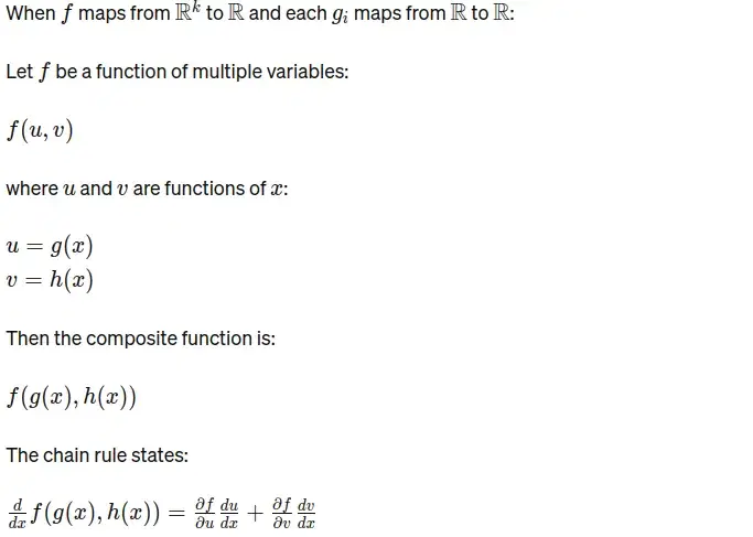
The chain rule is a fundamental concept in calculus used to find the derivative of composite functions. When dealing with functions of multiple variables, the chain rule helps us understand how a change in one variable affects another through a sequence of dependencies.
The General Chain Rule

Since functions in neural networks are scalar-valued, we need to discuss the chain rule specifically for scalar-valued functions.
Scalar-Valued Functions

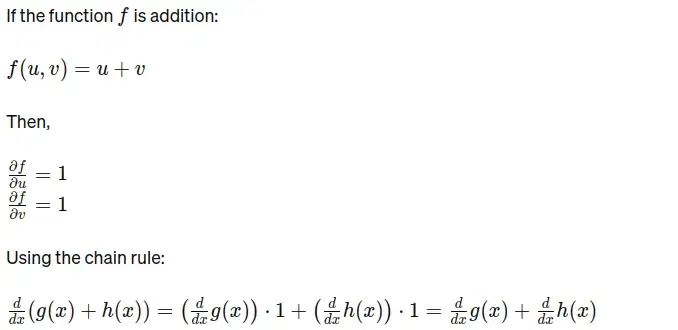
If you look at our __mul__ and __add__ functions, when we add or multiply two Value objects, we are creating a new function that is a composition of the two functions involved in the addition or multiplication. Here is an example of a chain rule involving a function that is a composite of two functions that are adding and multiplying with each other.
Addition

In the above examples of the chain rule u and v are parent functions or parent nodes and f is the children function or children node.
In the above code, the _backward() function calculates the derivative with respect to self and other. out is a composite of self and other, or out is a child of self and other. Since self and other are being added, the arithmetic operation is addition. According to the chain rule, the partial derivative will be 1 for all parent functions or variables when the arithmetic operation is addition. Therefore, the _backward() function is:
As the impact of multiplication by 1 is negligible, it is not explicitly included in the original code snippet. The question then arises: why do we multiply the partial derivatives of the parents (self and other) by the gradient of the child node (out.grad)? The answer lies in the chain rule. According to the chain rule, if a child node depends on its parent nodes, the effect of any change in the child node propagates to its parents. We calculate this effect by multiplying the gradient of the child by the gradients of the parents.
Now, why do we increment the gradients of the parents (self and other)? This is because if a parent node has more than one child, the effect of changes related to each child should be reflected in the gradient of the parent. According to the chain rule, this is achieved by adding each gradient. Thus, the gradients of self and other are incremented to accumulate the effects of all their children.
Multiplication

def __mul__(self, other):
other = other if isinstance(other, Value) else Value(other)
out = Value(self.data * other.data, (self, other), '*')
def _backward():
self.grad += other.data * out.grad
other.grad += self.data * out.grad
out._backward = _backward
return out
In the above code, the _backward() function calculates the derivative with respect to self and other. out is a composite of self and, or out is a child of self and other. Since self and other are being multiplied, the arithmetic operation is multiplication. According to the chain rule, the partial derivative of self will be other, and the partial derivative of other will be self.
The reason why we multiply the partial derivatives of self and other by out.grad and why we increment self.grad and other.grad is explained above.
Topological Sort:
Topological sort is a linear ordering of vertices in a Directed Acyclic Graph (DAG) such that for every directed edge u→v, vertex u comes before vertex v. This sorting is crucial in scenarios where certain tasks must be performed before others, such as task scheduling, course prerequisite planning, and, in our context, the sequence of computations in neural networks for backpropagation.
Role of Topological Sort in Backpropagation
Backpropagation is the process of computing the gradient of the loss function with respect to each parameter in the neural network. It involves moving backward through the computational graph of the network, starting from the output and working toward the input. Topological sort ensures that each node (representing a computation) is processed only after all its dependencies have been handled. This is essential because the gradient of each node depends on the gradients of its children.
Example Workflow
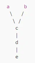
The topological graph of the above equations is given below.

The topological sort of the above graph would be: [a, b, c, d, e]. Because the backpropagation works in the opposite direction that is why will need topological sort in reverse order. The code below implements topological sort using the BFS method.
Explanation
The backward function uses Depth-First Search (DFS) to perform the topological sort that is necessary for backpropagation.
Initialization:
topo is an empty list that will store the nodes in topologically sorted order.
visited is a set used to keep track of visited nodes to avoid processing the same node multiple times.
build_topo Function
- This is a recursive function that performs a depth-first traversal of the graph.
- If a node v has not been visited, it is marked as visited.
- The function recursively visits all the nodes in v._prev (i.e., the parent nodes of v), exploring as far down each branch as possible before backtracking.
- After visiting all its parent nodes, v is appended to the topo list.
Topological Sort
The function build_topo(self) initiates the depth-first search from the current node (self), ensuring that all nodes influencing self are visited and ordered correctly in topo.
Backward Pass
- The gradient of the final output node (self) is initialized to 1.
- The nodes are processed in reverse topological order, starting from the output node and moving backward through the graph.
- The _backward method for each child node is called to propagate its gradient to its parents according to the chain rule.
I have explained the important functions related to backpropagation. Now, I will briefly explain the other functions of the Value class. But first I will explain double underscore (dunder) functions in python.
Double Underscore Functions in Python
Double underscore functions in Python, also known as 'dunder' methods (short for 'double underscore'), are special methods that have double underscores before and after their names (e.g., __init__, __add__). These methods are part of Python's data model and are used to define the behavior of objects for built-in operations. Functions __add__ and __mul__ which we have explained above are examples of 'dunder' functions in these functions we are defining the behavior of addition and multiplication for Value class.Let's move toward other functions of Value class.
Power Function (__pow__)
Explanation:
Purpose
This function allows a Value object to be raised to a power (exponentiation).
Parameters
- self: The current Value object.
- other: The exponent, which must be an integer or float.
Forward Pass
- The data attribute of self is raised to the power of other.
- A new Value object, out, is created with the result of the exponentiation. This new object keeps track of self as its parent, and the operation performed (exponentiation) is recorded.
Backward Pass
- The _backward function calculates the gradient of the exponentiation operation using the chain rule.
- The partial derivative is calculated according to the power rule of the derivative which is given below.
- This derivative is multiplied with out.grad to propagate the gradient backward.
Return
The function returns the new Value object out that represents the result of the exponentiation.
ReLU Function (relu)
Explanation:
Purpose
This function applies the ReLU (Rectified Linear Unit) activation function, which is commonly used in neural networks.
Mathematical Definition
The ReLU function is defined as: ReLU(x)=max(0,x)
This means:
- If the input x is greater than 0, the output is x.
- If the input x is less than or equal to 0, the output is 0.
Forward Pass
- The data attribute of self is compared to 0.
- If self.data is less than 0, out.data is set to 0.
- Otherwise, out.data is set to self.data.
- A new Value object, out, is created to store the result of the ReLU operation, keeping track of self as its parent and the operation performed (ReLU).
Backward Pass
- The _backward function calculates the gradient of the ReLU operation using the chain rule.
- The derivative of ReLU is 1 if self.data is greater than 0, and 0 otherwise.
- This derivative is multiplied by out.grad to propagate the gradient backward.
Return
- The function returns the new Value object out that represents the result of the ReLU activation.
- Purpose: This method allows the unary negation operator (-) to be used with Value objects. This function will help us to tackle subtraction as a special case of addition. It is used in __sub__ method of value class.
- Explanation: When -self is called, it returns the result of multiplying the Value object by -1. This effectively negates the value.
- Purpose: This method allows the addition operator (+) to be used with Value objects on the right-hand side.
- Explanation: __add__ method which is defined above is forself+ other.When other + self is called and other does not have its own __add__ method that can handle the addition, Python falls back to __radd__. This method simply calls self + other, leveraging the existing __add__ method.
- Purpose: This method allows the subtraction operator (-) to be used with Value objects.
- Explanation: When self - other is called, it returns the result of adding self to the negation of other. This is done using the previously defined __neg__ method.
- Purpose: This method allows the multiplication operator (*) to be used with Value objects on the right-hand side.
- Explanation: When other * self is called and other does not have its own __mul__ method that can handle the multiplication, Python falls back to __rmul__. This method simply calls self * other, leveraging the existing __mul__ method.
- Purpose: This method allows the true division operator (/) to be used with Value objects.
- Explanation: When self / other is called, it returns the result of multiplying self by the reciprocal of other. It handles division as a special case of multiplication. This uses the exponentiation operator (**) to raise other to the power of -1.
- Purpose: This method allows the true division operator (/) to be used with Value objects on the right-hand side.
- Explanation: When other / self is called and other does not have its own __truediv__ method that can handle the division, Python falls back to __rtruediv__. This method returns the result of multiplying other by the reciprocal of self.
- Purpose: This method provides a string representation of the Value object.
- Explanation: When repr(self) or print(self) is called, it returns a string that includes the data and grad attributes of the Value object. This is useful for debugging and logging purposes.
Why __radd__ and __rmul__ Are Needed
The __radd__ and __rmul__ methods (and other right-hand side methods like __rsub__ and __rtruediv__) are required to handle cases where the left operand does not support the operation with the Value object as the right operand. These methods ensure that the Value object can interact correctly with non-Value objects in binary operations.
Example Scenario
Consider the addition operation 3 + value_object, where value_object is an instance of the Value class.
Without __radd__
- Python first tries to call the __add__ method on the integer 3, but the integer class does not know how to handle a Value object.
- This results in a TypeError.
With __radd__
- When Python cannot find a suitable __add__ method on the left operand (the integer 3), it looks for an __radd__ method on the right operand (the Value object).
- The __radd__ method on the Value object is called, successfully handling the operation and returning the correct result.
We have gone through the code of Value class. Now I will explain the whole backpropagation process with an example.
Example
Let's consider the equations provided:
- c = a+b
- d = a×b
- f = c+d
Forward Pass
Perform addition and multiplication:
Perform addition to get e:
The computational graph is given below.

Backward Pass
Initialize Gradient for e:
The gradient for e with respect to e will be 1.
Process Each Node in Reverse Topological Order
The backward method computes the gradients in the correct order:
For e:
e is the composite function of c and d. The arithmetic operation between parent nodes is addition. So the partial derivative with respect to parent nodes will be 1.
- e._backward() propagates e.grad (which is 1) to c and d.
- c.grad += e.grad → c.grad = 1
- d.grad += e.grad → d.grad = 1
For d:
d is a composite function of a and b. The arithmetic operation between parent nodes is multiplication. So partial derivative with respect to a will be b and partial derivative with respect to b is a.
- d._backward() propagates d.grad to a and b.
- a.grad += b.data * d.grad → a.grad += 3.0 * 1 → a.grad = 3
- b.grad += a.data * d.grad → b.grad += 2.0 * 1 → b.grad = 2
For c:
d is a composite function of a and b. The arithmetic operation between parent nodes is addition. So the partial derivative with respect to parent nodes will be 1.
Due to the effect of d a.grad = 3
The computational graph after backpropagation is given below.
b.grad = 2
- c._backward() propagates c.grad to a and b
- a.grad += c.grad → a.grad += 1 → a.grad = 4
- b.grad += c.grad → b.grad += 1 → b.grad = 3

nn.py
To understand this file basic knowledge of neural network architecture is necessary. First I will explain neural network architecture.
Neural NetworksBackpropagationDeep LearningPythonMachine Learning